08: Fitting groups of electrodes

Read a real recording, clean it, fit every electrode, test which ones respond, and write the methods.

Introduction

The earlier tutorials fitted one made-up curve at a time. Here we use a real recording, with many electrodes, and do every step ourselves, in the order a study does them:

1. read the trials around each stimulation;

2. remove the artifact, the large electrical jump of the pulse itself;

3. re-reference, so that each electrode is compared with a good “zero”;

4. correct the baseline, so that each trial starts at zero;

5. check the trials, and flag the bad ones;

6. fit the average of each electrode;

7. test which electrodes really respond;

8. write the methods, the paragraph that tells readers what was done.

At the end, we see that one function, run_pipeline, does steps 2 to 7 at once with the settings of the preset.

The data

The recording comes from the Utrecht CCEP dataset (van Blooijs et al., 2023; OpenNeuro ds004080, free to use, CC0). Patients with epilepsy had electrodes placed on the brain before surgery. Two neighbouring electrodes were given short electrical pulses, one every 5 seconds, and the other electrodes recorded the answer of the brain: a CCEP (cortico-cortical evoked potential). Its first bump, the N1, comes between 9 and 50 ms; a slower one, the N2, between 50 and 300 ms.

The dataset is stored in BIDS, a common way to arrange brain recordings in folders and tables. We read one patient, one run, and the 10 pulses given to the electrode pair PT13-PT14.

import matplotlib.pyplot as plt
import numpy as np
import pandas as pd

import evoparam
from evoparam import plots, reports
from evoparam.artifact import remove_artifact
from evoparam.existence import test_response
from evoparam.io import read_bids
from evoparam.prep import baseline_correct, reject_trials, rereference

1. Reading the trials

read_bids finds the stimulation times in the events table of the dataset, and cuts a piece of recording around each one: a trial (also called an epoch). With remote=True, it reads straight from OpenNeuro, and only the few seconds it needs: about 15 MB here, instead of the whole 2 GB file.

• select keeps the pulses given to one electrode pair;

• picks keeps the electrodes we want: here the 46 electrodes of the grid (PT01 to PT48), without the two that were stimulated (they carry a huge artifact and no usable response);

• epoch is the piece kept around each pulse: from 1 s before to 1 s after.

site = "PT13-PT14"
picks = [f"PT{number:02d}" for number in range(1, 49) if f"PT{number:02d}" not in site]

trials = read_bids(
    "ds004080",
    "ccepAgeUMCU01",
    session="1",
    task="SPESclin",
    run="021448",
    remote=True,
    select={"stim_site": site},
    picks=picks,
    epoch=(-1.0, 1.0),
)
print(trials)

<TrialSet | 10 trials × 46 channels × 1024 times, -1.000 - 0.998 s, 512 Hz, uV, human, spes>

trials is a TrialSet: 10 trials × 46 electrodes × 1024 time points, from -1 s to +1 s, recorded 512 times per second (512 Hz), in µV. Time 0 is the pulse.

It also keeps a table with one row per trial (trials.metadata): when each pulse came, where, and how strong. evoparam gives the columns the same names for every dataset (stim_site, stim_current_mA…), whatever names the dataset used.

print(trials.metadata[["onset", "stim_site", "stim_current_mA"]].head(3))

         onset  stim_site  stim_current_mA
0  4015.720703  PT13-PT14              7.0
1  4020.720703  PT13-PT14              7.0
2  4025.720703  PT13-PT14              7.0

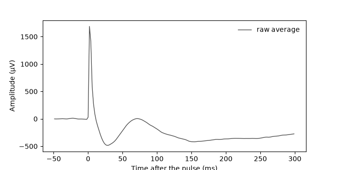
Here is the average of the 10 trials on electrode PT21, before any cleaning. We look from -50 to +300 ms.

def show_average(ts, channel, ax, label, color, start=-50, stop=300):
    """Draw the average of the trials of one electrode, in thin lines with a white edge."""
    times = ts.times * 1000
    keep = (times >= start) & (times <= stop)
    curve = ts.data[:, ts.ch_names.index(channel)].mean(axis=0)
    ax.plot(times[keep], curve[keep], color="white", linewidth=2.2)
    ax.plot(times[keep], curve[keep], color=color, linewidth=1.0, label=label)
    ax.set_xlabel("Time after the pulse (ms)")
    ax.set_ylabel("Amplitude (µV)")


fig, ax = plt.subplots(figsize=(7, 3.5))
show_average(trials, "PT21", ax, "raw average", "0.3")
ax.legend(frameon=False)

<matplotlib.legend.Legend object at 0x7f6a054cc910>

The very high and narrow peak at 0 ms is the artifact: the electrical pulse itself, picked up by the electrode. It is much larger than the brain response. Right after it, the curve dips down to about -480 µV near 28 ms: that is the N1 we want to measure. Then comes a slower dip after 100 ms, the N2.

2. Removing the artifact

remove_artifact takes the pulse out of every trial. With method="template", it builds the typical shape of the artifact (the template: here the median of the 10 trials), scales it to each trial and electrode, and subtracts it, in a short window around the pulse (window, from -2 to +8 ms).

After the pulse, the recording equipment takes a few ms to settle: a slow tail that fades away. tail="joint" leaves this tail to the fit, which models it as the background (tutorial 01), together with the bumps.

The baseline is a piece of the trial before the pulse, with no response in it: here from -500 to -20 ms. It tells the method what “no artifact” looks like.

cleaned = remove_artifact(
    trials,
    method="template",
    window=(-0.002, 0.008),
    tail="joint",
    baseline=(-0.5, -0.02),
    random_state=0,
)

print(np.round(cleaned.quality, 2))

[0.62 0.62 0.61 0.62 0.62 0.62 0.62 0.62 0.61 0.62]

cleaned holds the cleaned trials (cleaned.cleaned) and a quality score for each trial: how well the artifact was removed, from 0 (badly) to 1 (very well).

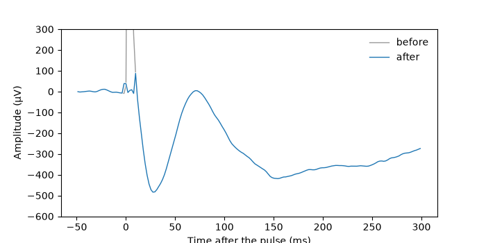
The figure compares the average before and after.

fig, ax = plt.subplots(figsize=(7, 3.5))
show_average(trials, "PT21", ax, "before", "0.6")
show_average(cleaned.cleaned, "PT21", ax, "after", "C0")
ax.set_ylim(-600, 300)
ax.legend(frameon=False)

<matplotlib.legend.Legend object at 0x7f6a054fa0d0>

The jump at 0 ms is gone: only small wiggles are left in the first 8 ms, where the samples of the window were replaced. Outside the window the two curves are the same (the grey one is hidden under the blue one), and the N1 near 28 ms is untouched.

Note

The window ends at 8 ms, 1 ms before the fit starts (9 ms): the artifact removal never touches the part of the curve that we measure.

3. Re-referencing

A voltage is always measured between two points: the electrode and a reference. If the reference picks up activity, every electrode gets it too. Re-referencing changes the reference after the recording.

A common choice is the common average: subtract, at each time point, the mean of all electrodes. But the electrodes that respond would then put their response into that mean, and into every other electrode. "car_adaptive" (adjusted common average) first finds the electrodes with no response in 10-300 ms, and averages only those.

referenced = rereference(cleaned.cleaned, "car_adaptive", random_state=0)

print(referenced.provenance.steps[-1]["settings"]["members"])

['PT01', 'PT02', 'PT03', 'PT05', 'PT06', 'PT09', 'PT10', 'PT11', 'PT17', 'PT18', 'PT19', 'PT20', 'PT25', 'PT26', 'PT27', 'PT28', 'PT29', 'PT30', 'PT31', 'PT32', 'PT33', 'PT34', 'PT35', 'PT36', 'PT37', 'PT38', 'PT39', 'PT40', 'PT41', 'PT42', 'PT45', 'PT46', 'PT47', 'PT48']

34 of the 46 electrodes were judged quiet and used for the average; the 12 others were left out of it (each one still gets the average subtracted).

4. Correcting the baseline

Each trial starts at its own level: the brain’s slow waves move it up or down. We subtract, from each trial and electrode, its mean over the baseline (-500 to -20 ms). All trials then sit around zero before the pulse, and the average is not pulled up or down by a few of them.

ready = baseline_correct(referenced, (-0.5, -0.02))

5. Checking the trials

A trial can be bad: the patient moved, an electrode came loose, the artifact was badly removed. reject_trials looks for trials that are much larger, much noisier or flatter than the others, or that have a low artifact quality score.

It looks at each trial on each electrode. A trial that is odd on one electrode only is masked on that electrode: the average of that electrode leaves it out. A trial that is odd on half of the electrodes or more is rejected everywhere.

It never deletes anything: it adds columns to metadata: rejected (True or False), reject_reason and n_flagged_channels (on how many electrodes the trial was masked).

checked = reject_trials(ready, baseline=(-0.5, -0.02))
print(checked.metadata[["rejected", "n_flagged_channels"]])

   rejected  n_flagged_channels
0     False                   0
1     False                   0
2     False                  12
3     False                   2
4     False                   0
5     False                   0
6     False                   3
7     False                   9
8     False                   2
9     False                   0

No trial is rejected, but a few trials are masked on some electrodes: trial 2 on 12 electrodes, trial 7 on 9. On PT21, for example, the average now uses 9 trials out of 10. Masking changes the averages a little, and so the numbers of the fit.

6. Fitting each electrode

evoparam.fit averages the trials of each electrode, then fits the average, as fit_response did in the earlier tutorials, with the settings of the preset. It gives back a GroupFit: one fit per electrode.

group = evoparam.fit(checked, "ccep", random_state=0)

table = group.to_dataframe()
n1 = table[table["label"] == "N1"]
print(n1[["channel", "latency", "amplitude"]].round(3).to_string(index=False))

channel  latency  amplitude
   PT05    0.041   -289.237
   PT07    0.037   -389.543
   PT15    0.026   -272.401
   PT18    0.031   -129.254
   PT21    0.032   -475.350
   PT22    0.022   -143.976
   PT23    0.037   -122.605
   PT24    0.034  -1714.117
   PT26    0.049   -111.998
   PT30    0.027   -129.782
   PT32    0.033   -151.704
   PT34    0.049   -195.135
   PT42    0.038   -156.584
   PT43    0.024    -30.752

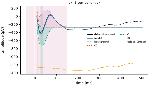
14 electrodes have an N1. The latency is in seconds (0.032 s = 32 ms) and the amplitude in µV. On PT21, the N1 comes at 32 ms with -475 µV.

The amplitude of a bump is measured from the background, not from zero, so it is not exactly the lowest point of the curve.

group.get("PT03") gives the fit of one electrode, which can be read and drawn like the fits of the earlier tutorials.

fit = group.get("PT21")
fig = plots.plot_fit(fit)

Note

PT24 has an N1 of -1714 µV, much larger than the others. Such a value is worth a look (plots.plot_fit(group.get("PT24"))) before you trust it: close to the stimulated pair, what is left of the artifact and its tail can add to a bump.

7. Testing which electrodes respond

A fit always finds something, even in pure noise. To decide if an electrode really responds, test_response asks: is the curve after the pulse (9-500 ms) larger than what the noise alone would give?

The noise alone is made by sign flips: each trial is randomly turned upside down or not, many times (1000 here). A real response, the same at every trial, cancels out when half of the trials are flipped; noise does not change. If the real curve is larger than almost all the flipped ones, the electrode responds.

The answer is a p-value: the chance of a curve this large from noise alone. Small is good. Since we test 46 electrodes, some would pass by luck; the p-values are corrected for this (correction="fdr_bh", the default), and an electrode responds when its corrected p-value is below 0.05.

The test is run on all the trials (ready, before the masks of step 5), as run_pipeline does below.

test = test_response(ready, window=(0.009, 0.5), baseline=(-0.5, -0.02), by=(), random_state=0)
answer = pd.DataFrame(
    {
        "channel": test.settings["channels"],
        "p_value": np.ravel(test.p_value),
        "responds": np.ravel(test.significant),
    }
)
print(answer.round(3).to_string(index=False))

channel  p_value  responds
   PT01    0.386     False
   PT02    0.054     False
   PT03    0.054     False
   PT04    0.016      True
   PT05    0.016      True
   PT06    0.039      True
   PT07    0.039      True
   PT08    0.016      True
   PT09    0.140     False
   PT10    0.208     False
   PT11    0.039      True
   PT12    0.016      True
   PT15    0.016      True
   PT16    0.017      True
   PT17    0.080     False
   PT18    0.208     False
   PT19    0.566     False
   PT20    0.017      True
   PT21    0.017      True
   PT22    0.018      True
   PT23    0.028      True
   PT24    0.016      True
   PT25    0.090     False
   PT26    0.189     False
   PT27    0.370     False
   PT28    0.230     False
   PT29    0.801     False
   PT30    0.370     False
   PT31    0.090     False
   PT32    0.132     False
   PT33    0.801     False
   PT34    0.040      True
   PT35    0.140     False
   PT36    0.998     False
   PT37    0.393     False
   PT38    0.071     False
   PT39    0.162     False
   PT40    0.255     False
   PT41    0.663     False
   PT42    0.158     False
   PT43    0.156     False
   PT44    0.310     False
   PT45    0.801     False
   PT46    0.355     False
   PT47    0.393     False
   PT48    0.094     False

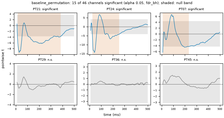
15 of the 46 electrodes respond. The test and the fit answer two different questions, so they do not always agree:

• 8 electrodes respond and have an N1 (PT05, PT07, PT15, PT21, PT22, PT23, PT24, PT34);

• 7 respond without an N1 (PT04, PT06, PT08, PT11, PT12, PT16, PT20): their response is later, or its dip in 9-50 ms is not deep enough;

• 6 have an N1 but do not pass the test (PT18, PT26, PT30, PT32, PT42, PT43): a dip is there in the average, but it does not stand out enough from trial to trial.

Most studies keep the N1 of an electrode only when the electrode also passes the test.

The figure shows, for each electrode, the test statistic over time (a measure of how far the curve is from zero, compared with its spread over trials) and the band where noise alone stays.

fig = plots.plot_existence(test, channels=["PT21", "PT24", "PT07", "PT29", "PT36", "PT45"])

All the steps at once

Steps 2 to 7 are the chain of the "ccep" preset, with its own settings: same artifact window, same reference, same baseline, same test. reports.run_pipeline runs this chain in one call, from the raw trials.

result = reports.run_pipeline(trials, "ccep", random_state=0, trial_fits=False)
table_all = result.group.to_dataframe()
print(table_all[table_all["label"] == "N1"][["channel", "latency", "amplitude"]].round(3))

   channel  latency  amplitude
8     PT05    0.032   -145.720
11    PT06    0.017   -128.931
15    PT07    0.037   -389.543
20    PT08    0.035  -1112.413
32    PT15    0.026   -272.401
43    PT18    0.031   -129.254
47    PT21    0.028   -354.120
55    PT23    0.037   -122.605
58    PT24    0.038   -918.300
64    PT26    0.049   -111.998
69    PT30    0.027   -129.782
71    PT31    0.032    -97.376
74    PT32    0.033   -151.704
78    PT34    0.049   -195.135
79    PT35    0.048   -118.772
88    PT42    0.038   -156.584
90    PT43    0.024    -28.895

run_pipeline does not mask any trial (step 5 is not part of the preset’s chain), so its averages use all 10 trials, and its numbers are those of steps 2-4 and 6 without the masks. It finds 17 N1 instead of 14, and on PT21 the N1 comes at 28 ms with -354 µV, instead of 32 ms and -475 µV. With only 10 trials, leaving one out is enough to move a bump: this is why every choice of cleaning goes in the methods.

Doing the steps one by one is useful to look at each of them; run_pipeline is shorter, and it is sure to use the preset’s settings everywhere.

trial_fits=False skips the fit of each single trial, which the preset does too but which takes longer.

8. The methods paragraph

Every step above wrote down what it did, with all its settings. reports.methods_text turns this into the paragraph of the “Methods” section of a paper: what was done, in what order, with which values, and what to cite.

print(reports.methods_text(result.results))

Evoked responses were analysed with evoparam (version 0.1.0.dev0) using the preset 'ccep' v1.2; validation: ds004080 (REQ-113, REQ-114, REQ-135). The stimulation artifact was removed by template subtraction (evoparam.artifact.remove_artifact, method 'template') in the window -2 to 8 ms (global template; templates grouped by the metadata columns stim_site, stim_current_mA and stim_polarity (those present); scaled to each trial and channel; recovery tail left to the response model and fitted jointly with its background). A quality score between 0 and 1 was computed for every trial. Channels were re-referenced to an adjusted common average from which channels with a response were excluded (responses judged in 10 to 300 ms). Each trial and channel was baseline-corrected by subtracting the mean of -500 to -20 ms of its own trial. Trials were averaged per channel (mean). In the window 9 to 500 ms, each waveform was modelled as an exponential background plus up to 6 components (skewed gaussian and gaussian; full width at half maximum 3 to 250 ms, both polarities). Amplitudes and background coefficients were solved by variable projection and the other parameters by bounded least squares (linear loss, 3 starts). Components were added one at a time and kept when the BIC decreased by at least 10, computed on residuals whitened by an autoregressive model of the noise of the plus-minus average of the trials (alternating signs, whole epoch). A final model holding two overlapping components of opposite sign was refitted from starts on the extrema of the data and replaced when the refit was better; a component of the refitted model that no longer lowered the criterion by the same amount was removed. Uncertainty: Jacobian-based (Wald) intervals at 95 %. Onset and offset are the times where a component reaches 10 % of its peak amplitude. Components were labelled by latency window: N1 (9 to 50 ms, negative), N2 (50 to 300 ms, negative) and delayed (100 to 1000 ms, either polarity). A response was said to have an N1 when the fitted curve (background and components) had a negative peak in 9 to 50 ms deeper than 3.4 times the noise standard deviation estimated by the fit. Classical measures (peak, mean amplitude, area and fractional-area latencies) were computed on the same window. The presence of a response in 9 to 500 ms was tested on every channel with a sign-flip permutation test of the trials (max_t statistic, 1000 permutations) against the baseline -500 to -20 ms (both polarities, alpha = 0.05, Benjamini-Hochberg false-discovery-rate correction across channels). Random draws used the seed 0; the result can be regenerated from its recorded provenance with evoparam.reproduce. Software: Bellec Y.V. evoparam: parameterizing evoked neural responses (version 0.1.0). https://github.com/yannbellec/evoparam Methods: Benjamini and Hochberg (1995) for the false-discovery-rate correction.

Read it and adapt it to your paper, but do not change the numbers: they are the ones that were used. The last sentence says how to make the same result again (evoparam.reproduce), from the record that each result keeps.

Note

Try it yourself: change site to another pair of the same run (look at trials.metadata without select to see them), or keep other electrodes in picks. Each time, compare the electrodes with an N1 and the ones that pass the test.

Conclusion

A real analysis goes: read the trials (read_bids), remove the artifact (remove_artifact), re-reference (rereference), correct the baseline (baseline_correct), flag bad trials (reject_trials), fit each electrode (evoparam.fit), test which ones respond (test_response) and write the methods (reports.methods_text). reports.run_pipeline does the steps of the preset in one call. Look at the figures at each step: a number is only as good as the curve under it.

Data: van Blooijs D, van den Boom MA, van der Aar JF, et al. Developmental trajectory of transmission speed in the human brain. Nature Neuroscience 26, 689-700 (2023). OpenNeuro ds004080, CC0.