16: Time-frequency responses

Parameterise induced oscillatory bursts into zones, data-driven or from a published atlas.

Introduction

Not every response shows up in the average curve. An induced response is an oscillation whose phase is random from trial to trial: it adds power at some frequency and time, but it averages to nearly zero, so the tutorials so far would miss it. You see it only in the power of single trials, on a time-frequency map.

evoparam.tf parameterises that map. Instead of one number per pixel, it finds a few zones: rectangles in time and frequency where the power clearly rises or falls, each with a centre, an extent, a strength and a p-value. Two ways to get the zones:

1. data-driven: let evoparam find the zones from the map itself (NMF);

2. published: score the exact zones a paper defined, for example the Brinyark 2026 atlas (theta, alpha, beta, low and high gamma, in an N1 and an N2 window).

It also removes the trap where a sharp evoked N1 leaks broadband power into high gamma: the fitted N1 is subtracted first, so a high-gamma zone is a real oscillation, not the edge of a spike.

import warnings

from evoparam import plots
from evoparam.sim import simulate_bursts
from evoparam.tf import list_published_zones, tf_fit

The data

simulate_bursts adds induced bursts to noise, with a known truth. Each burst is a cosine under a smooth envelope, at a given frequency, centre time and duration, with a random phase per trial (so it is invisible in the average). We put two bursts on one channel: a beta burst (20 Hz) early, and a high-gamma burst (120 Hz) later.

bursts = [
    {"freq": 20.0, "centre": 0.15, "duration": 0.15, "amplitude": 25.0, "channel": 0},
    {"freq": 120.0, "centre": 0.25, "duration": 0.12, "amplitude": 30.0, "channel": 0},
]
trials, truth = simulate_bursts(
    40, n_channels=1, sfreq=1000.0, bursts=bursts, noise_sd=10.0, seed=0,
)  # fmt: skip
print(trials)

<TrialSet | 40 trials × 1 channels × 1400 times, -0.600 - 0.799 s, 1000 Hz, uV, human, erp>

Data-driven zones

tf_fit first makes the time-frequency map (a Morse wavelet by default), normalises it against the baseline in decibels, and keeps only the pixels that beat a permutation test. With zones="auto" it then factorises the significant map into a few zones. freqs is (low, high, n): here 4 to 250 Hz in 32 steps.

with warnings.catch_warnings():
    warnings.simplefilter("ignore")
    tf = tf_fit(trials, freqs=(4, 250, 32), zones="auto", max_zones=4,
                n_permutations=500, random_state=0)  # fmt: skip

columns = [
    "zone_id",
    "freq_centroid",
    "freq_extent",
    "time_centroid",
    "p_value",
    "energy_fraction",
]
print(tf.zones[columns].round(3).to_string(index=False))

zone_id  freq_centroid  freq_extent  time_centroid  p_value  energy_fraction
      0         20.482        0.354           0.15    0.000            0.518
      1        127.914        0.287           0.25    0.000            0.479
      2         65.860        0.000           0.66    0.001            0.001

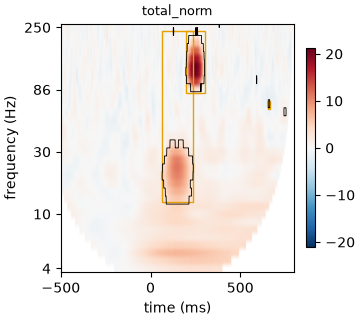
The two bursts come back as two zones: one near 20 Hz around 150 ms, one in high gamma around 250 ms. freq_centroid and time_centroid are where each zone sits, energy_fraction is how much of the significant power it holds, and p_value is its significance under the permutation null. The figure shows the total map, the N1-corrected footprint and the residual.

fig = plots.plot_tf(tf)

Published zones

When a paper defines fixed zones, score those exact boxes instead of finding your own. list_published_zones is the registry; the Brinyark 2026 atlas splits the map into theta, alpha, beta, low gamma and high gamma, each in an early (N1) and a late (N2) window.

zones = list_published_zones()
zone_columns = ["name", "f_low", "f_high", "t_start", "t_end", "verified"]
print(zones[zone_columns].head(6).to_string(index=False))

                           name  f_low  f_high  t_start  t_end  verified
brinyark2026_delayed_high_gamma   50.0   250.0    0.050   0.50      True
              brinyark2026_GhN2   50.0   250.0    0.050   0.50      True
               brinyark2026_TN1    4.0     8.0    0.015   0.05     False
               brinyark2026_TN2    4.0     8.0    0.050   0.50     False
               brinyark2026_AN1    8.0    13.0    0.015   0.05     False
               brinyark2026_AN2    8.0    13.0    0.050   0.50     False

Pass zones="published:<name>" to score one. Our 120 Hz burst at 250 ms sits in the delayed high-gamma zone (brinyark2026_GhN2: 50 to 250 Hz, 50 to 500 ms). The zones table gives the box, and zone_metrics gives what was measured inside it: the power value (dB), a t-statistic, a p_value and the fraction of the box that is significant.

with warnings.catch_warnings():
    warnings.simplefilter("ignore")
    tf_pub = tf_fit(trials, freqs=(4, 250, 32), zones="published:brinyark2026_GhN2",
                    n_permutations=500, random_state=0)  # fmt: skip

box_columns = ["zone_id", "f_low", "f_high", "t_start", "t_end"]
print(tf_pub.zones[box_columns].round(3).to_string(index=False))
print()
metrics = ["zone", "channel", "value", "t", "p_value", "fraction_significant"]
print(tf_pub.zone_metrics[metrics].round(4).to_string(index=False))

 zone_id  f_low  f_high  t_start  t_end
       0   50.0   250.0     0.05    0.5

             zone channel  value       t  p_value  fraction_significant
brinyark2026_GhN2      c0 1.2412 16.4361      0.0                0.1076

Note

Only the delayed-high-gamma zone is marked verified in the registry; the others are read from the article but not yet checked against evoparam’s own recovery test, so they need allow_unverified=True. tf_compare contrasts the maps of two conditions with a cluster test, and tf_fit(..., by_trial=True) gives the zone power per trial, to correlate with dose, distance or behaviour as in tutorial 09.

Conclusion

Time-frequency parameterisation finds the responses that the average hides: induced bursts of power. tf_fit turns the map into a few zones with timing, frequency and a p-value, either data-driven or from a published atlas, and it subtracts the fitted N1 first so a high-gamma zone is a true oscillation and not the leakage of a sharp evoked peak.